3 連立一次方程式(消去法)
3.1 連立方程式の表現方法
連立1次方程式(Linear Equations)は,次のような形をしている.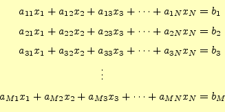
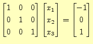
式(7)は行列とベクトルで書くと,式がすっきりして 考えやすくなる.書き直すと,
である.それぞれの行列とベクトルは,
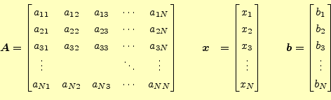 |
を表す.
通常,連立1次方程式(7)は
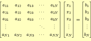
と書き表せる.このようにすると,見通しがかなり良くなる.
3.2 ガウス・ジョルダン法の基本的な考え方
ガウス・ジョルダン(Gauss-Jordan)法というのは,連立方程式 (10)を次にように変形させて,解く方法である.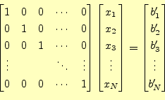 |
この式から明らかに,求める解
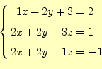
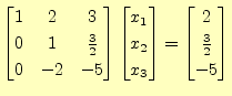
をガウス・ジョルダン法で解を求める. 解くべき,方程式
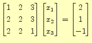 |
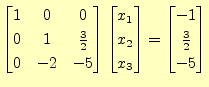
2行
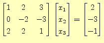 |
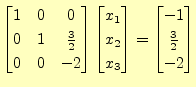
3行
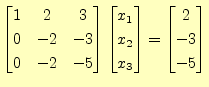 |
 |
1行
 |
3行
 |
 |
 |
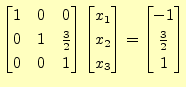
これで,ガウス・ジョルダン法による対角化の作業は完了である.これか ら,
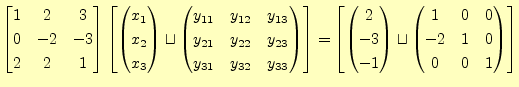
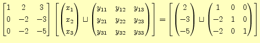
3.3 逆行列
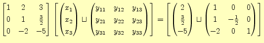
ガウス・ジョルダンを使って,逆行列が求められる.以下のようにする.解くべき,方程式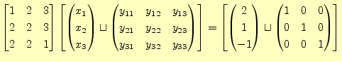 |
とする.
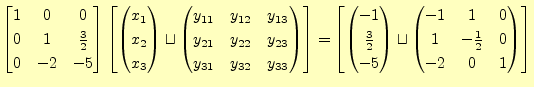
2行![]() 1行
1行
 |
3行
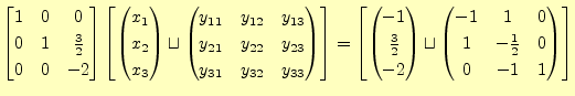
 |
 |
1行
 |
3行
 |
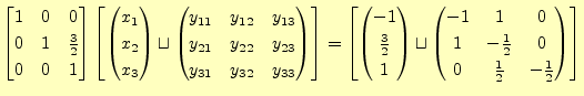 |
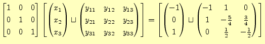 |
これで,ガウス・ジョルダン法による対角化の作業は完了である.これか ら,
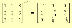 |
と分かる.
3.4 ガウス・ジョルダン法のC言語の関数
ピボット選択は行わないで,逆行列も求めないのガウス・ジョルダン法で連立方程式を計 算するプログラムを示す.このプログラムの動作は,次の通りである.- 仮引数「n」は,解くべき連立方程式の未知数の数である.
- 仮引数の配列「a」と「b」は,係数行列
 と非同次項
と非同次項
 である.
値は,呼び出し元からにアドレス渡しで送られる.
である.
値は,呼び出し元からにアドレス渡しで送られる.
- 係数行列は,配列「a[1][1]」〜「a[n][n]」に格納されている.
- 非同次項は,配列「b[1]」〜「b[n]」に格納されている.
- 連立方程式の解
 は,配列「b[1]」〜「b[n]」に格納される.
- このプログラムでの処理が終了すると,配列「a[1][1]」〜「a[n][n]」は単位 行列になる..
	/* ========== ガウスジョルダン法の関数 =================*/
	void gauss_jordan(int n, double a[][100], double b[]){

	   int ipv, i, j;
	   double inv_pivot, temp;

	   for(ipv=1 ; ipv <= n ; ipv++){

	      /* ---- 対角成分=1(ピボット行の処理) ---- */
	      inv_pivot = 1.0/a[ipv][ipv];
	      for(j=1 ; j <= n ; j++){
	         a[ipv][j] *= inv_pivot;
	      }
	      b[ipv] *= inv_pivot;

	      /* ---- ピボット列=0(ピボット行以外の処理) ---- */
	      for(i=1 ; i<=n ; i++){
	         if(i != ipv){
	            temp = a[i][ipv];
	            for(j=1 ; j<=n ; j++){
	               a[i][j] -= temp*a[ipv][j];
	            }
	            b[i] -= temp*b[ipv];
	         }
	      }

	   }
	}
ホームページ: Yamamoto's laboratory
著者: 山本昌志 Yamamoto Masashi
平成18年11月27日