2 電気回路

2.1 回路素子

フーリエ変換を使って，図1-3の基本的な回路素子のインピーダン スを考えよう．諸君はこれらの回路素子の時間領域における基本的な動作の知識しかない-- とする．回路の動作を表す時間領域の微分方程式から，周波数領域--正確には角振動数 領域--の方程式に直して，周波数領域のインピーダンスを求めることにする．したがっ て，インピーダンスは$\omega$の関数で，

$$Z(\omega)=\cfrac{\tilde{V}(\omega)}{\tilde{I}(\omega)}$$ (9)

と定義する．ここで， $\tilde V(\omega)$は周波数領域の電圧

$$\tilde{V}(\omega)=\frac{1}{\sqrt{2\pi}} \int_{-\infty}^{\infty}V(t)e^{-i\omega t}\,\mathrm{d}t$$ (10)

$\tilde I(\omega)$は周波数領域の電流

$$\tilde{I}(\omega)=\frac{1}{\sqrt{2\pi}} \int_{-\infty}^{\infty}I(t)e^{-i\omega t}\,\mathrm{d}t$$ (11)

である．

図 1: レジスタンス

図 2: インダクタンス

図 3: キャパシタンス

2.1.1 抵抗

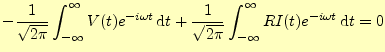
図1の回路を計算することにより，抵抗の周波数領域のインピーダンスを求め る．電流に関するキルヒホッフの法則は自動的に満たしている．電圧に関するキルヒホッフの法則より，

$$-V(t)+RI(t)=0$$ (12)

となる．両辺に $e^{-i\omega t}$両辺を乗じて，区間 $[-\infty,\,\infty]$で$t$につい て積分を行う．すると，

$$-\frac{1}{\sqrt{2\pi}}\int_{-\infty}^\infty V(t)e^{-i\omega t}\,\... ... +\frac{1}{\sqrt{2\pi}}\int_{-\infty}^\infty RI(t)e^{-i\omega t}\,\mathrm{d}t=0$$ (13)

が得られる．これは，フーリエ変換なので，

$$-\tilde{V}(\omega)+R\tilde{I}(\omega)=0$$ (14)

と書いてもよい．この式から，直ちに

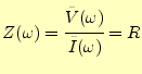$$Z(\omega)=\cfrac{\tilde{V}(\omega)}{\tilde{I}(\omega)}=R$$ (15)

が得られる．普通の抵抗(registance)は，周波数に依存しない．

2.1.2 インダクタンス

つぎに，図2の回路を計算することにより，インダクタンスの周波数領域のイ ンピーダンスを求める．インダクタンスは，電流が増加すると電流を流さないように逆に 電圧が発生する．発生する電圧は，電流の変化率に比例し，インダクタンス$L$の大きさ にも比例する．電流の流れる方向を図2のようにして，インダクタンスの下か ら上方向を正の電圧とすると，

$$V_L(t) =L\lim_{\varDelta t\to 0}\frac{I(t+\varDelta t)-I(t)}{\varDelta t}$$

$$=L \if 11 \frac{\,\mathrm{d}I(t)}{\,\mathrm{d}t} \else \frac{\,\mathrm{d}^{1} I(t)}{\,\mathrm{d}t^{1}}\fi$$ (16)

となる．

図2の回路の電圧に関するキルヒホッフの法則は，

$$-V(t)+V_L(t)=0$$ (17)

となる．先の式から，

$$-V(t)+L \if 11 \frac{\,\mathrm{d}I(t)}{\,\mathrm{d}t} \else \frac{\,\mathrm{d}^{1} I(t)}{\,\mathrm{d}t^{1}}\fi =0$$ (18)

である．先ほど同様に，両辺をフーリエ変換する．ここで，導関数のフーリエ変換を使う と，

$$-\tilde{V}(\omega)+i\omega L\tilde{I}(\omega)=0$$ (19)

となる．したがって，この回路のインピーダンスは，

$$Z(\omega)=\cfrac{\tilde{V}(\omega)}{\tilde{I}(\omega)}=i\omega L$$ (20)

である．インピーダンスは周波数に依存するのである．

2.1.3 キャパシタンス

つぎに，図3の回路を計算することにより，キャパシタンスの周波数領域のイ ンピーダンスを求める．キャパシタンスは，電極に電荷が貯ると電圧が発生する．発生す る電圧は，電荷量に比例し，静電容量$C$にも反比例する．電荷の方向を図3の ようにして，キャパシタンスの下から上方向を正の電圧とすると，

$$V_C(t) =\frac{Q(t)}{C}$$ (21)

となる．

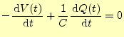
図3の回路の電圧に関するキルヒホッフの法則は，

$$-V(t)+V_C(t)=0$$ (22)

となる．先の式から，

$$-V(t)+\frac{Q(t)}{C}=0$$ (23)

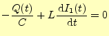
である．電流の関数を使いたいが，電荷の関数となっている．電荷から電流に直すために， 両辺を時間で微分する．

$$- \if 11 \frac{\,\mathrm{d}V(t)}{\,\mathrm{d}t} \else \frac{\,\ma... ...(t)}{\,\mathrm{d}t} \else \frac{\,\mathrm{d}^{1} Q(t)}{\,\mathrm{d}t^{1}}\fi =0$$ (24)

これは，

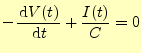$$- \if 11 \frac{\,\mathrm{d}V(t)}{\,\mathrm{d}t} \else \frac{\,\mathrm{d}^{1} V(t)}{\,\mathrm{d}t^{1}}\fi +\frac{I(t)}{C}=0$$ (25)

と書き直すことができる．電流と電荷の方向を図3のように決めたならば，

$$\if 11 \frac{\,\mathrm{d}Q(t)}{\,\mathrm{d}t} \else \frac{\,\mathrm{d}^{1} Q(t)}{\,\mathrm{d}t^{1}}\fi =I(t)$$ (26)

の関係があるからである．

先ほど同様に，両辺をフーリエ変換する．ここで，導関数のフーリエ変換を使うと，

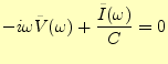$$-i\omega\tilde{V}(\omega)+ \frac{\tilde{I}(\omega)}{C}=0$$ (27)

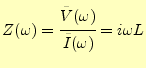
となる．したがって，この回路のインピーダンスは，

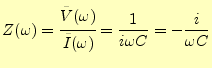$$Z(\omega)=\cfrac{\tilde{V}(\omega)}{\tilde{I}(\omega)}=\frac{1}{i\omega C}=-\frac{i}{\omega C}$$ (28)

である．この場合もまた，インピーダンスは周波数に依存するのである．

2.2 直列・並列回路

つぎに，図4と図5の回路を考える．

図 4: LC直列回路

図 5: LC並列回路

2.2.1 直列回路

図4の回路を表す電圧に関するキルヒホッフの法則は，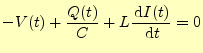

$$-V(t)+\frac{Q(t)}{C}+L \if 11 \frac{\,\mathrm{d}I(t)}{\,\mathrm{d}t} \else \frac{\,\mathrm{d}^{1} I(t)}{\,\mathrm{d}t^{1}}\fi =0$$ (29)

である．両辺を時間$t$で微分し， $\,\mathrm{d}Q(t)/\,\mathrm{d}t=I(t)$を使うと，

$$- \if 11 \frac{\,\mathrm{d}V(t)}{\,\mathrm{d}t} \else \frac{\,\ma... ...(t)}{\,\mathrm{d}t} \else \frac{\,\mathrm{d}^{2} I(t)}{\,\mathrm{d}t^{2}}\fi =0$$ (30)

が得られる．両辺をフーリエ変換すると，

$$-i\omega\tilde{V}(\omega) +\frac{\tilde{I}(\omega)}{C} +(i\omega)^2 L\tilde{I}(\omega)=0$$ (31)

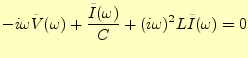
がえられる．これを整理すると，

$$i\omega\tilde{V}(\omega)= \left[ \frac{1}{C}+(i\omega)^2 L \right]\tilde{I}(\omega)$$ (32)

となる．これから，電源からみた回路のインピーダンスは，

$$Z(\omega) =\cfrac{\tilde{V}(\omega)}{\tilde{I}(\omega)}$$

$$=\frac{1}{i\omega C}+i\omega L$$

$$=i\omega L-\frac{i}{\omega C}$$ (33)

となる．

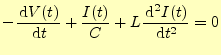
2.2.2 並列回路

図4の回路を表す電圧に関するキルヒホッフの法則は，

$$-V(t)+\frac{Q(t)}{C}=0$$ (34)

$$-\frac{Q(t)}{C}+L \if 11 \frac{\,\mathrm{d}I_1(t)}{\,\mathrm{d}t} \else \frac{\,\mathrm{d}^{1} I_1(t)}{\,\mathrm{d}t^{1}}\fi =0$$ (35)

である．それぞれの式の両辺を微分すると，

$$- \if 11 \frac{\,\mathrm{d}V(t)}{\,\mathrm{d}t} \else \frac{\,\ma... ...(t)}{\,\mathrm{d}t} \else \frac{\,\mathrm{d}^{1} Q(t)}{\,\mathrm{d}t^{1}}\fi =0$$ (36)

$$-\frac{1}{C} \if 11 \frac{\,\mathrm{d}Q(t)}{\,\mathrm{d}t} \else ... ...)}{\,\mathrm{d}t} \else \frac{\,\mathrm{d}^{2} I_1(t)}{\,\mathrm{d}t^{2}}\fi =0$$ (37)

が得られる．ここで， $\,\mathrm{d}Q(t)/\,\mathrm{d}t$はキャパシタンス中に流れる電流で，

$$\if 11 \frac{\,\mathrm{d}Q(t)}{\,\mathrm{d}t} \else \frac{\,\mathrm{d}^{1} Q(t)}{\,\mathrm{d}t^{1}}\fi =I(t)-I_1(t)$$ (38)

となる．これを，式(36)と(37)に代入すると，

$$- \if 11 \frac{\,\mathrm{d}V(t)}{\,\mathrm{d}t} \else \frac{\,\mathrm{d}^{1} V(t)}{\,\mathrm{d}t^{1}}\fi +\frac{1}{C}\left[I(t)-I_1(t)\right]=0$$ (39)

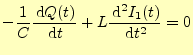
$$\frac{1}{C}\left[-I(t)+I_1(t)\right]+L \if 12 \frac{\,\mathrm{d}I... ...)}{\,\mathrm{d}t} \else \frac{\,\mathrm{d}^{2} I_1(t)}{\,\mathrm{d}t^{2}}\fi =0$$ (40)

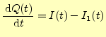
である．これらの連立方程式をフーリエ変換すると

$$-i\omega\tilde{V}(\omega)+\frac{1}{C}\left[\tilde{I}(\omega)-\tilde{I}_1(\omega)\right]=0$$ (41)

$$\frac{1}{C}\left[-\tilde{I}(\omega)+\tilde{I}_1(\omega)\right]+L(i\omega)^2\tilde{I}_1(\omega)=0$$ (42)

が得られる．この連立方程式から，電源から見たインピーダンスの計算に不要な $\tilde{I}_1(\omega)$を消去すると，

$$\frac{1}{C}\left[-\tilde{I}(\omega)-i\omega C\tilde{V}(\omega)+\t... ...ight]+ L(i\omega)^2\left[-i\omega C\tilde{V}(\omega)+\tilde{I}(\omega)\right]=0$$ (43)

が得られる．整理すると，

$$\left(1-\omega^2LC\right)\tilde{V}(\omega)-i\omega L\tilde{I}(\omega)=0$$ (44)

となる．したがって，電源から見たインピーダンスは，

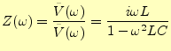$$Z(\omega)=\frac{\tilde{V}(\omega)}{\tilde{V}(\omega)}=\frac{i\omega L}{1-\omega^2LC}$$ (45)

となる．

2.2.2.1 電気回路風

通常の電気回路の問題と同じになることを確かめよう．これは並 列回路なので，インピーダンスは，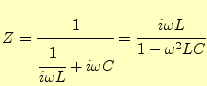

$$Z=\cfrac{1}{\cfrac{1}{i\omega L}+i\omega C}=\cfrac{i\omega L}{1-\omega^2 LC}$$ (46)

となる．フーリエ変換を使って求めたインピーダンスと一致する．世の中，うまくできて いる．
ホームページ: Yamamoto's laboratory
著者: 山本昌志